Future Leaked Covariate Importance in Synthefy Foundation Model using Zero-Perturbation Analysis
In this walkthrough, we demonstrate how to estimate the influence of leaked covariates by zero-perturbing them only at inference time. In this work, we generate synthetic autoregressive-with-exogenous-input (ARX) time-series data and demonstrate that Zero-Perturbation Analysis appropriately assigns scores based on the usefulness of the data. We show how to:- ✅ Run a perturbation experiment using sMAPE
- ✅ Visualize how forecasts change when each covariate is removed
- ✅ Aggregate importance across 100 simulation runs
🔍 Goal
Which external covariates does the model actually rely on for forecasting?The core tool we utilize is Zero-Perturbation Analysis: for each covariate, mask the entire covariate, both history and future leaked, by replacing it with zero, and compare the prediction error (sMAPE) for this data point. If the model depends heavily on a covariate, removing it will hurt the forecast.
🧪 1) Synthetic ARX Data
We simulate data from an ARX(3,4) model with four exogenous inputs: with Gaussian noise . This is a linear function of the history and the exogenous inputs, which are sampled from random Fourier functions with orders between 3-20. Note that we can generate a near-infinite variety of ARX(3,4) time series by sampling different exogenous inputs. Output columns:| Column | Description |
|---|---|
yt | target time series |
x1–x4 | exogenous inputs (MixedSampler) |
time | integer index (optional) |
⚙️ 2) Prepare History / Forecast Split
We split the series into history and forecast horizon (default 80/20).🧯 3) Zero-Perturbation Protocol & sMAPE Shift
For each covariate , we zero it over both the history and forecast horizon (no retraining) and measure the relative sMAPE shift as a percentage: Intuitively, this metric indicates how much the performance dropped relative to the overall accuracy of the prediction, an indicator for how important the covariate is.- : removing hurts accuracy → model depends on it
- : removing helps or does nothing → likely redundant/noisy
📊 4) Single-Run “Summary” Plots
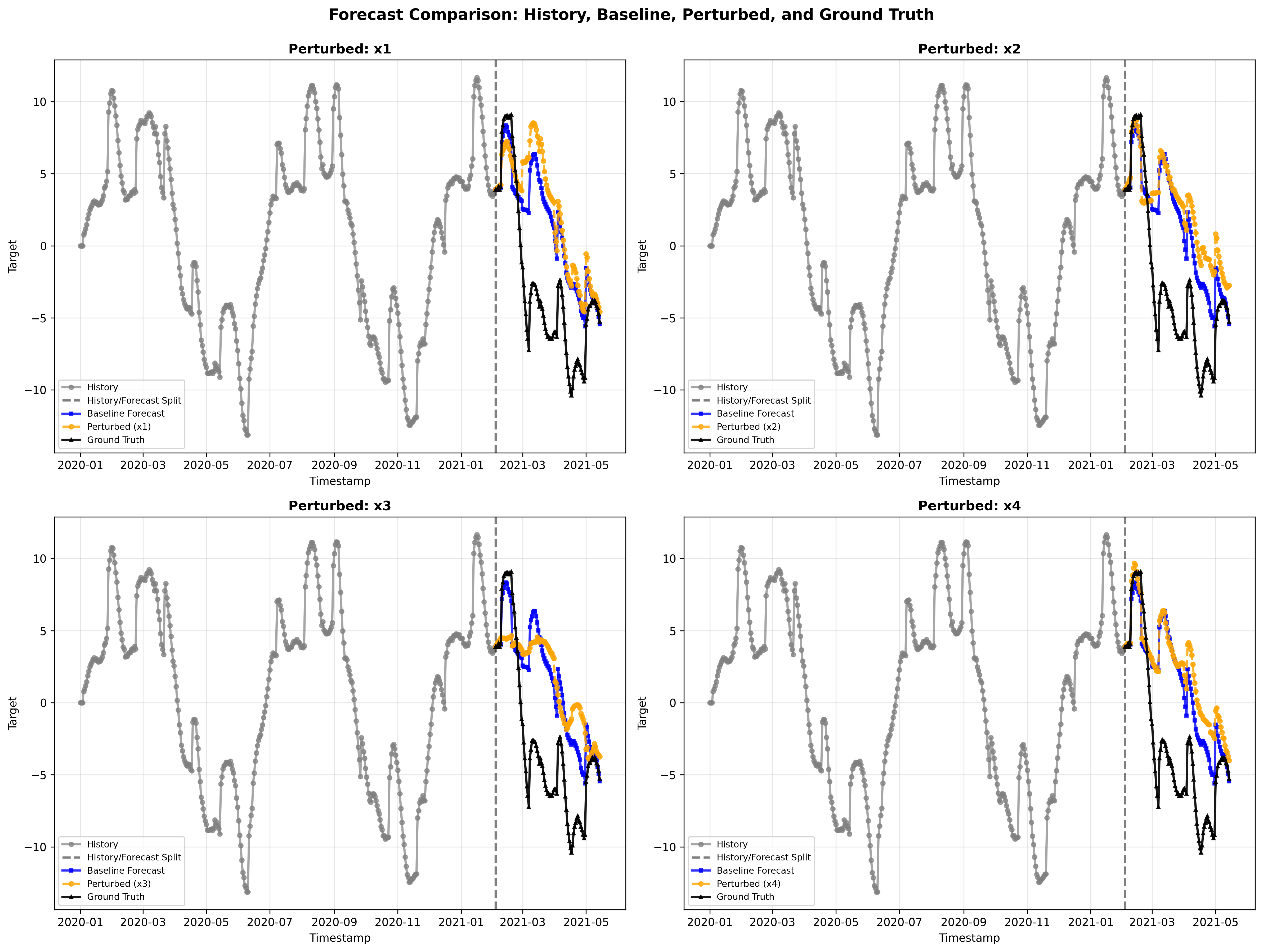
4.1 Forecast Comparison
We show the results of zero-perturbation for a randomly sampled ARX(3,4) time series. Each panel masks one covariate (x1–x4) using zero perturbation, replacing the covariate with a zero column (we only show the target time series):
- Blue = baseline forecast
- Orange = forecast with masked covariate
- Larger divergence ⇒ stronger dependence on that covariate
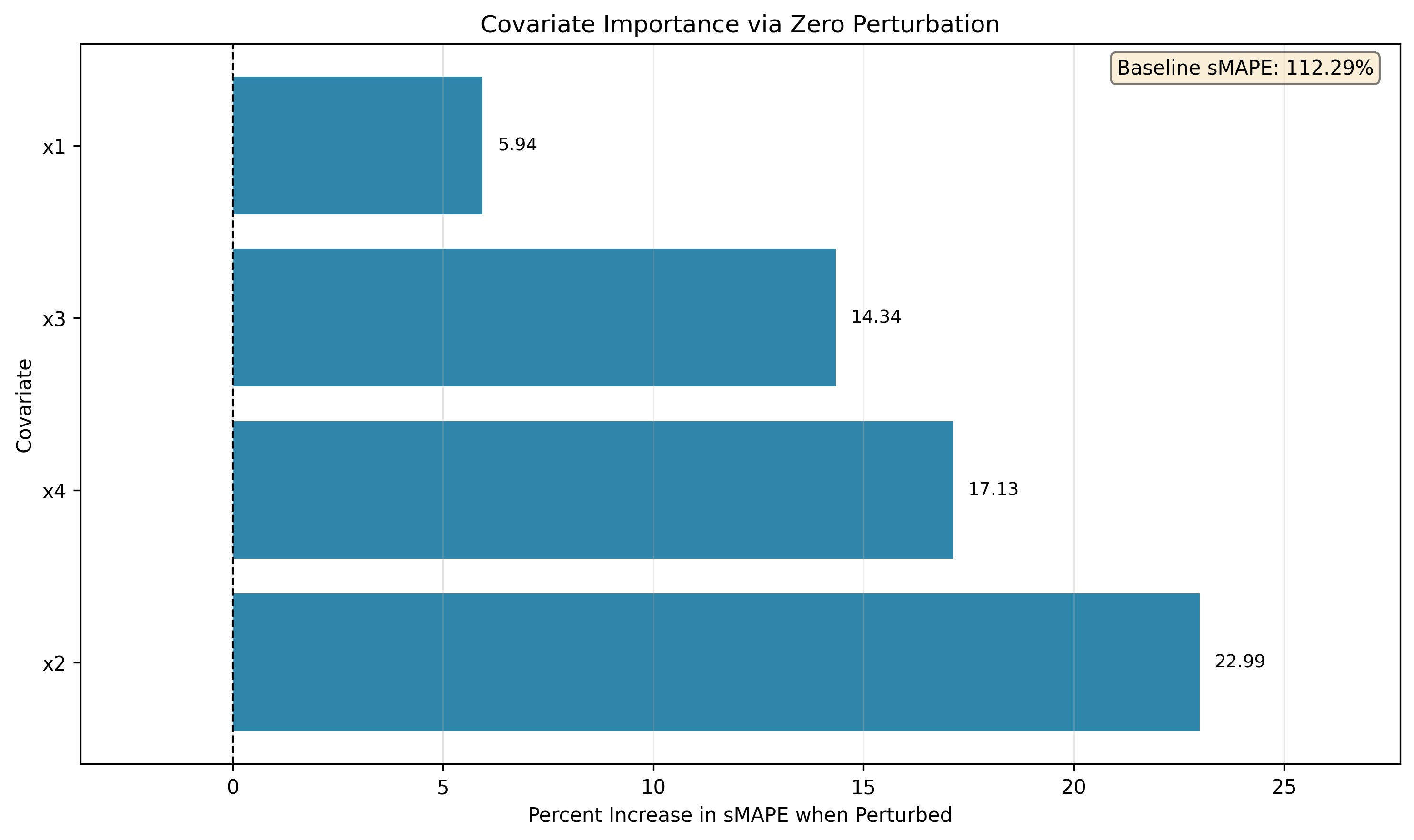
4.2 Per-Run Covariate Importance
| Covariate | Δ-sMAPE (%) |
|---|---|
| x1 | 5.94 |
| x2 | 22.99 |
| x3 | 14.34 |
| x4 | 17.13 |
🎲 5) Variability Across Seeds
Even though the ARX coefficients are kept constant, the exogenous signals are sampled randomly, producing variability across runs. We provide a sample from a different seed (resulting in different exogenous covariates) to indicate how this variability can affect the perturbation analysis on a per-run basis. This seed shows how variance can result in significantly different change in sMAPE from perturbation.5.1 Forecast Comparison

5.2 Importance
| Covariate | Δ-sMAPE (%) |
|---|---|
| x1 | 50.7 |
| x2 | 4.0 |
| x3 | -3.4 |
| x4 | 0.3 |
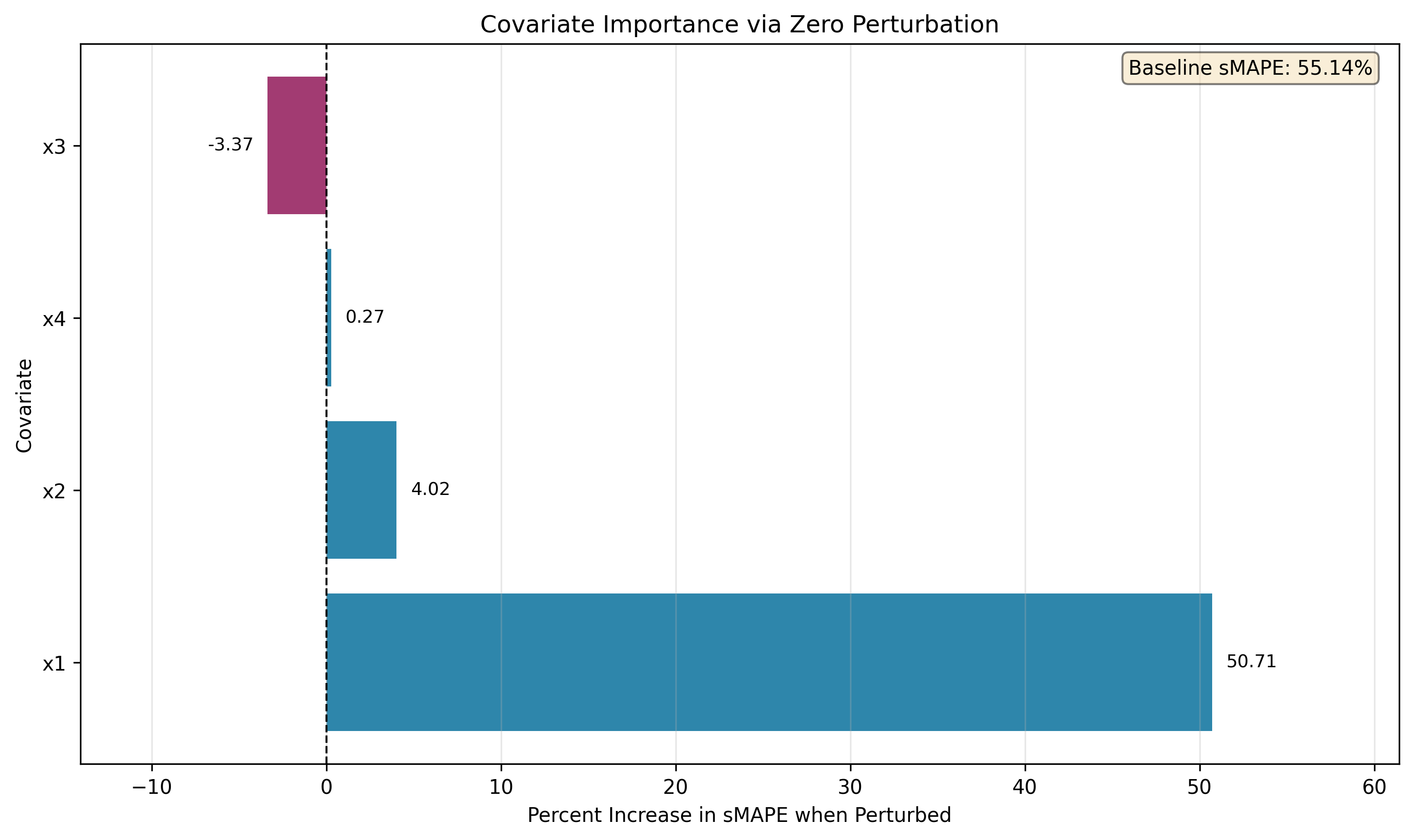
🧠 Single-run attribution is unreliable — use distributional analysis.
📈 6) Aggregated Statistics Across 100 Samples
Even though individual runs may have variation in the perturbation analysis, the aggregated trends indicate that Zero-perturbation offers an efficient and meaningful indication of covariate importance. In this experiment, we generated 100 samples of ARX(3,4) data, with the same coefficients as indicated in Section 1.6.1 Error-Shift Distributions
The error shift distribution indicates how often different relative sMAPE shift values occur across 100 samples. Notice that while skewed right (importance), there is quite a bit of variability and even negative (lower error after zero perturbation).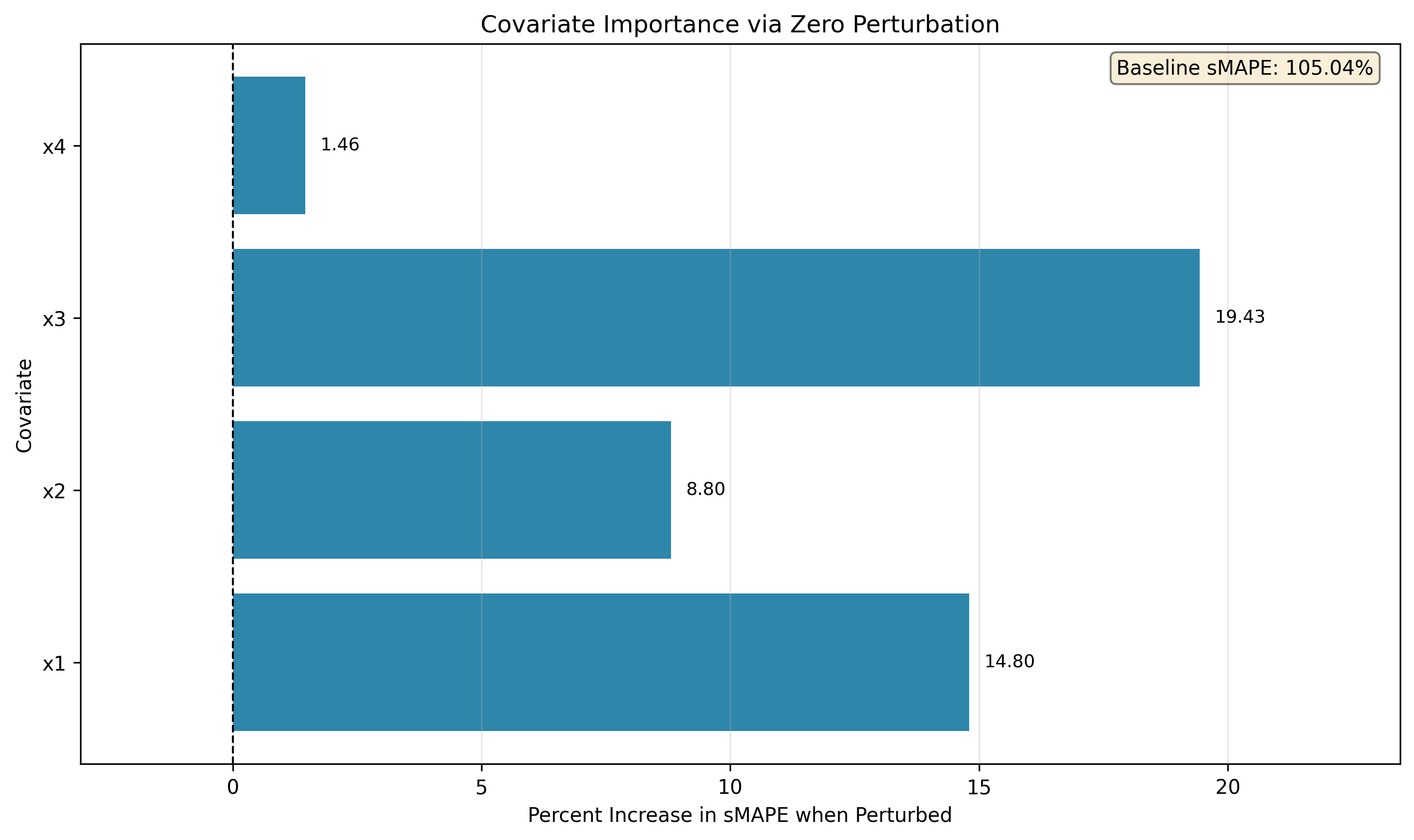
6.2 Mean Importance (Global Ranking)
Nonetheless, the aggregated importance is consistent with the weights of the ARX(3,4) data, indicating that zero perturbation is a good measure of covariate importance with sufficient data, correctly weighting the individual covariates according to their importance.✅ Key Takeaways
- Zero-perturbation is a fast, retraining-free alternative to SHAP/LIME for time series. Note that because SHAP/LIME requires significantly more calls to the model, they can be too costly for substantial analysis.
- Negative Importance can occur, indicative of unpredictability in the true forecast
- Histograms reveal risk profiles: there can be variability in benefit across samples
- ARX data allows us to pinpoint the current capabilities of the model.