Installation
Install the Synthefy Python package:Authentication
Set your API key as an environment variable (you can get your key here: https://console.synthefy.com/api-keys):Basic Forecasting
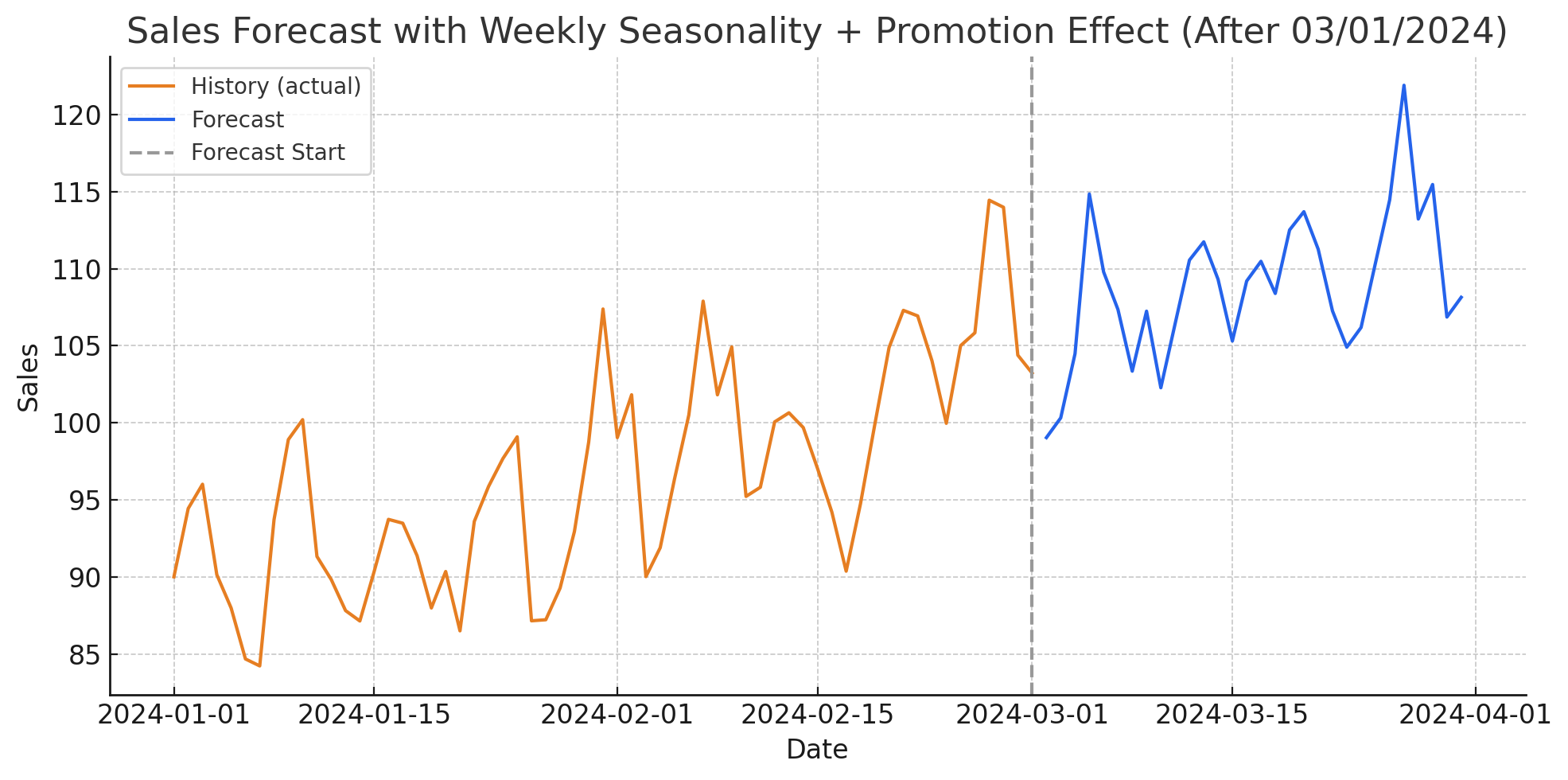
Simple Sales Forecast
Here’s a complete example of forecasting sales data. We’ll create historical data and then prepare it for forecasting:For complete documentation of the
forecast_dfs method, see the API Client documentation.basic_forecast.py
Show plotting code for historical analysis
Show plotting code for historical analysis
Using Leak Columns
When you have some knowledge about future information, like promotions, you can “leak” this data so our model can leverage it for the forecast.Backtesting
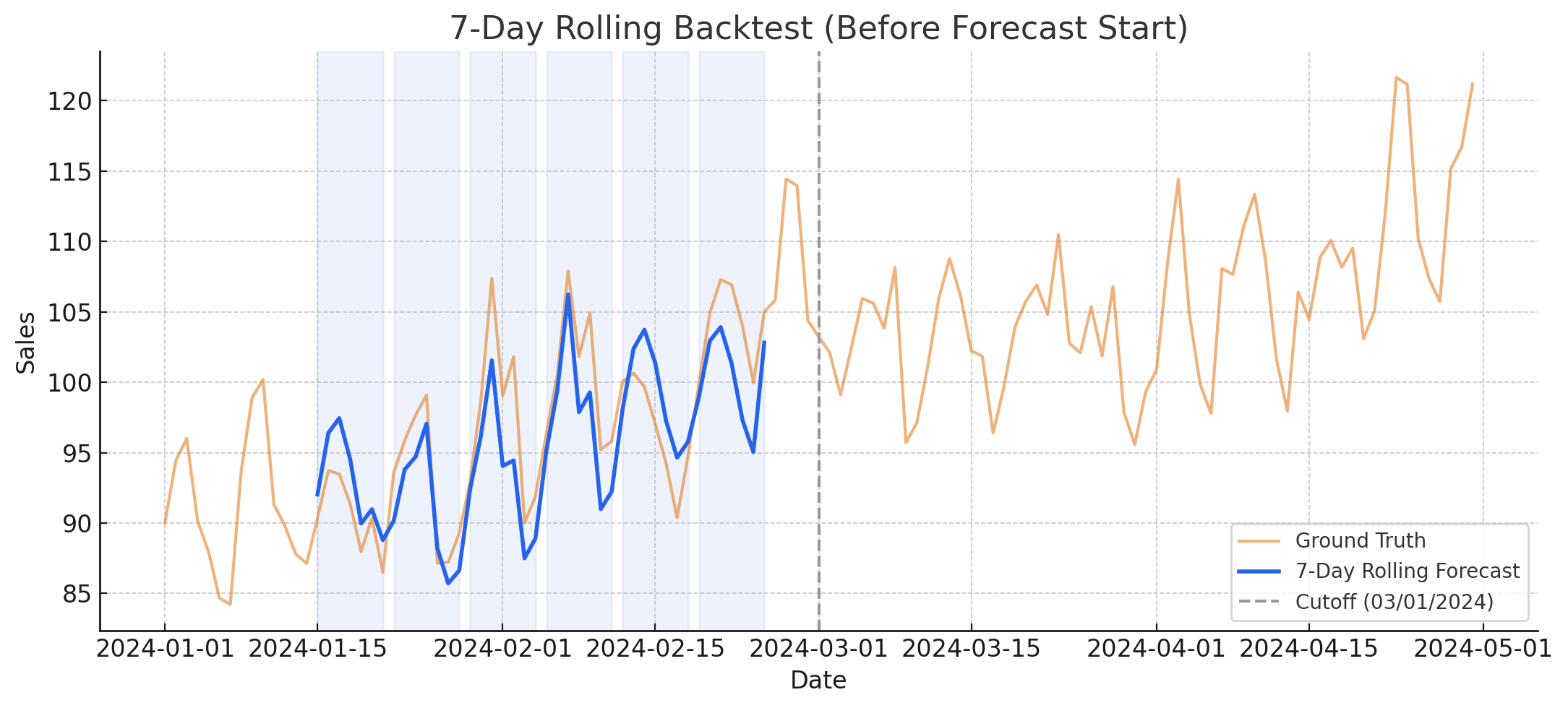
Example: 7-Day Rolling Forecasts
Here’s how to backtest with 7-day forecast windows, moving forward 7 days at a time. The API automatically handles splitting your data into multiple time windows:For complete documentation of the
from_dfs_pre_split method, see the ForecastV2Request documentation.backtest_example.py
Show plotting code for historical analysis
Show plotting code for historical analysis