> ## Documentation Index
> Fetch the complete documentation index at: https://docs.synthefy.com/llms.txt
> Use this file to discover all available pages before exploring further.
# Time Series Quickstart
> Get started with Synthefy's time series forecasting API in minutes.
Get started with Synthefy's powerful forecasting API in minutes. This guide will walk you through making your first forecast using our Python client.
## Installation
Install the Synthefy Python package:
```bash theme={null}
pip install synthefy
```
## Authentication
Set your API key as an environment variable (you can get your key here: [https://console.synthefy.com/api-keys](https://console.synthefy.com/api-keys)):
```bash theme={null}
export SYNTHEFY_API_KEY="your-api-key-here"
```
Or pass it directly to the client:
```python theme={null}
# For synchronous usage
from synthefy.api_client import SynthefyAPIClient
# For asynchronous usage
from synthefy.api_client import SynthefyAsyncAPIClient
```
## Basic Forecasting
### Simple Sales Forecast
Here's a complete example of forecasting sales data. We'll create historical data and then prepare it for forecasting:
```python basic_forecast.py theme={null}
import pandas as pd
import numpy as np
import asyncio
from synthefy.api_client import SynthefyAsyncAPIClient
async def main():
# Create your data
df = pd.DataFrame({
'date': pd.date_range('2024-01-01', periods=130, freq='D'),
'sales': np.random.normal(100, 10, 130) + np.sin(np.arange(130) * 2 * np.pi / 7) * 5,
'promotion_active': np.random.choice([0, 1], 130)
})
# Split your data into "what we know" vs "what we want to predict"
cutoff_date = '2024-03-15' # Everything before this date is history
# Historical data: what the model learns from
history_df = df[df['date'] <= cutoff_date].copy()
# Future data: what we want to forecast (with known metadata but unknown sales)
future_dates = pd.date_range('2024-03-16', periods=30, freq='D')
target_df = pd.DataFrame({
'date': future_dates,
'sales': np.nan, # We don't know future sales - this is what we want to predict!
'promotion_active': [1, 0, 0, 1, 0, 0, 1, 0, 0, 1] * 3 # Known future promotions
})
# Make the forecast
# The model uses historical sales + future metadata to predict future sales
async with SynthefyAsyncAPIClient() as client:
forecast_dfs = await client.forecast_dfs(
history_dfs=[history_df], # What we know (past sales + metadata)
target_dfs=[target_df], # What we want to predict (future sales)
target_col='sales', # The column we want to forecast
timestamp_col='date', # The time column
metadata_cols=['promotion_active'], # Additional context
leak_cols=[], # No columns with future information
model='Migas-1.0'
)
# Get your predictions
forecast_df = forecast_dfs[0]
print(forecast_df.head())
# Run the async function
asyncio.run(main())
```
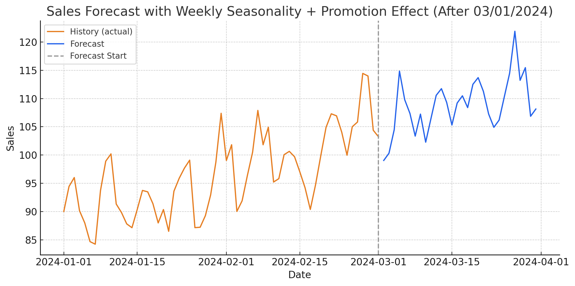
**Forecasting Reult**
```python theme={null}
# --- Plot: History vs Forecast ---
import matplotlib.pyplot as plt
# History up to cutoff
cutoff_ts = pd.to_datetime(cutoff_date)
hist_for_plot = history_df.copy()
# forecast_df is returned by Synthefy; it contains the predicted `sales` for the future dates
fig, ax = plt.subplots(figsize=(10, 5))
ax.plot(hist_for_plot["date"], hist_for_plot["sales"], label="History (actual)", color="#e67e22")
ax.plot(forecast_df["date"], forecast_df["sales"], label="Forecast", color="#2563eb")
ax.axvline(cutoff_ts, linestyle="--", color="#999", label="Forecast Start")
ax.set_title("Sales Forecast with Weekly Seasonality + Promotion Effect")
ax.set_xlabel("Date")
ax.set_ylabel("Sales")
ax.legend()
fig.tight_layout()
plt.show()
```
 ### Using Leak Columns
When you have some knowledge about future information, like promotions, you can "leak" this data so our model can leverage it for the forecast.
```python theme={null}
# Make forecast with leak columns
forecast_dfs = await client.forecast_dfs(
history_dfs=[history_df],
target_dfs=[target_df],
target_col='sales',
timestamp_col='date',
metadata_cols=['promotion_active'],
leak_cols=['promotion_active'],
model='Migas-1.0'
)
```
## Backtesting
### Example: 7-Day Rolling Forecasts
Here's how to backtest with 7-day forecast windows, moving forward 7 days at a time. The API automatically handles splitting your data into multiple time windows:
```python backtest_example.py theme={null}
import asyncio
import pandas as pd
import numpy as np
from synthefy.data_models import ForecastV2Request
from synthefy.api_client import SynthefyAsyncAPIClient
async def main():
# Create sample time series data
dates = pd.date_range('2023-01-01', '2023-03-31', freq='D')
data = {
'date': dates,
'sales': np.random.normal(100, 10, len(dates)),
'store_id': 1,
'category_id': 101,
'promotion_active': np.random.choice([0, 1], len(dates), p=[0.7, 0.3])
}
df = pd.DataFrame(data)
# Use from_dfs_pre_split for backtesting with date-based windows
request = ForecastV2Request.from_dfs_pre_split(
dfs=[df],
timestamp_col='date',
target_cols=['sales'],
model='Migas-1.0',
cutoff_date='2023-03-01', # Start backtesting from March 1st
forecast_window='7D', # 7-day forecast windows
stride='7D', # Move forward 7 days between windows
metadata_cols=['store_id', 'category_id', 'promotion_active'],
leak_cols=['promotion_active'] # Promotion data may leak into target
)
print(f"Created {len(request.samples)} forecast windows for backtesting")
print("Window details:")
for i, sample in enumerate(request.samples):
history_start = sample[0].history_timestamps[0]
history_end = sample[0].history_timestamps[-1]
target_start = sample[0].target_timestamps[0]
target_end = sample[0].target_timestamps[-1]
print(f" Window {i+1}: History {history_start} to {history_end}, Target {target_start} to {target_end}")
# Make async forecast request
async with SynthefyAsyncAPIClient() as client:
response = await client.forecast(request)
# Process results for each window
for i, forecast_row in enumerate(response.forecasts):
print(f"Window {i+1}: {len(forecast_row[0].timestamps)} forecast points")
# Access forecast values
if forecast_row[0].values:
print(f" Forecast values: {forecast_row[0].values[:3]}...") # First 3 values
# You can now compare these forecasts with actual values from df
# to calculate metrics like MAE, RMSE, etc.
asyncio.run(main())
```
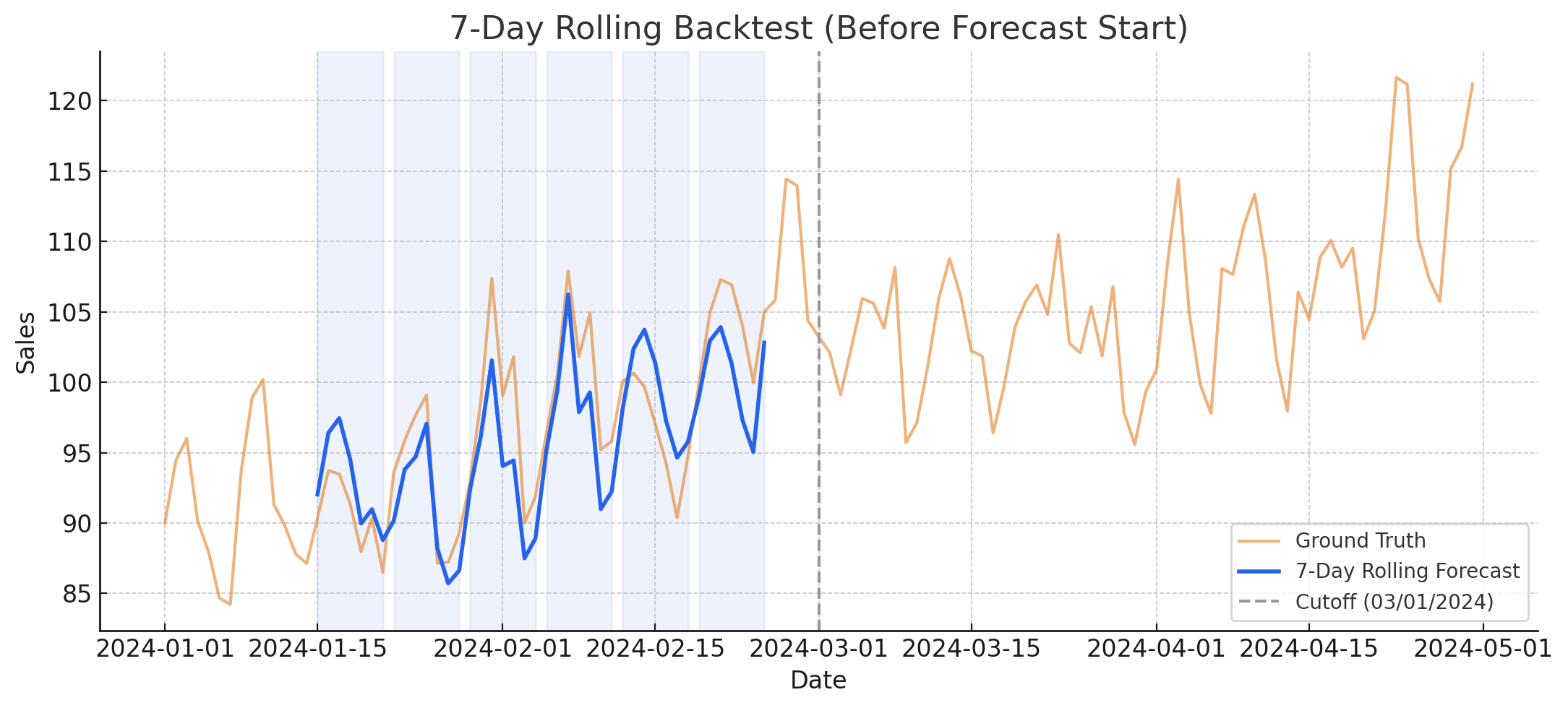
**Backtesting Reult**
```python theme={null}
# --- Plot: 7-Day Rolling Backtest windows vs Ground Truth ---
import matplotlib.pyplot as plt
# 1) Collect all window forecasts into a single dataframe
all_windows = []
for w in response.forecasts:
if w[0].timestamps and w[0].values:
wdf = pd.DataFrame({
"date": pd.to_datetime(w[0].timestamps),
"forecast": w[0].values,
})
all_windows.append(wdf)
if len(all_windows) == 0:
raise ValueError("No backtest forecast windows returned.")
backtest_df = pd.concat(all_windows, ignore_index=True)
# 2) Plot GT (entire df) + rolling window forecasts
cutoff_ts = pd.Timestamp("2023-03-01")
fig, ax = plt.subplots(figsize=(11, 5))
ax.plot(df["date"], df["sales"], color="#e67e22", alpha=0.6, label="Ground Truth")
ax.plot(backtest_df["date"], backtest_df["forecast"],
color="#2563eb", linewidth=2, label="7-Day Rolling Forecasts")
# Shade each 7-day target window (optional but helpful)
# windows are in `request.samples` in the same order as `response.forecasts`
for sample in request.samples:
tgt_start = pd.to_datetime(sample[0].target_timestamps[0])
tgt_end = pd.to_datetime(sample[0].target_timestamps[-1])
# Only shade windows that are <= cutoff (typical backtest setup)
if tgt_end <= cutoff_ts:
ax.axvspan(tgt_start, tgt_end, color="#2563eb", alpha=0.08)
ax.axvline(cutoff_ts, linestyle="--", color="#999", label="Cutoff (03/01/2023)")
ax.set_title("7-Day Rolling Backtest (Ground Truth vs Forecast)")
ax.set_xlabel("Date")
ax.set_ylabel("Sales")
ax.legend()
fig.tight_layout()
plt.show()
```
### Using Leak Columns
When you have some knowledge about future information, like promotions, you can "leak" this data so our model can leverage it for the forecast.
```python theme={null}
# Make forecast with leak columns
forecast_dfs = await client.forecast_dfs(
history_dfs=[history_df],
target_dfs=[target_df],
target_col='sales',
timestamp_col='date',
metadata_cols=['promotion_active'],
leak_cols=['promotion_active'],
model='Migas-1.0'
)
```
## Backtesting
### Example: 7-Day Rolling Forecasts
Here's how to backtest with 7-day forecast windows, moving forward 7 days at a time. The API automatically handles splitting your data into multiple time windows:
```python backtest_example.py theme={null}
import asyncio
import pandas as pd
import numpy as np
from synthefy.data_models import ForecastV2Request
from synthefy.api_client import SynthefyAsyncAPIClient
async def main():
# Create sample time series data
dates = pd.date_range('2023-01-01', '2023-03-31', freq='D')
data = {
'date': dates,
'sales': np.random.normal(100, 10, len(dates)),
'store_id': 1,
'category_id': 101,
'promotion_active': np.random.choice([0, 1], len(dates), p=[0.7, 0.3])
}
df = pd.DataFrame(data)
# Use from_dfs_pre_split for backtesting with date-based windows
request = ForecastV2Request.from_dfs_pre_split(
dfs=[df],
timestamp_col='date',
target_cols=['sales'],
model='Migas-1.0',
cutoff_date='2023-03-01', # Start backtesting from March 1st
forecast_window='7D', # 7-day forecast windows
stride='7D', # Move forward 7 days between windows
metadata_cols=['store_id', 'category_id', 'promotion_active'],
leak_cols=['promotion_active'] # Promotion data may leak into target
)
print(f"Created {len(request.samples)} forecast windows for backtesting")
print("Window details:")
for i, sample in enumerate(request.samples):
history_start = sample[0].history_timestamps[0]
history_end = sample[0].history_timestamps[-1]
target_start = sample[0].target_timestamps[0]
target_end = sample[0].target_timestamps[-1]
print(f" Window {i+1}: History {history_start} to {history_end}, Target {target_start} to {target_end}")
# Make async forecast request
async with SynthefyAsyncAPIClient() as client:
response = await client.forecast(request)
# Process results for each window
for i, forecast_row in enumerate(response.forecasts):
print(f"Window {i+1}: {len(forecast_row[0].timestamps)} forecast points")
# Access forecast values
if forecast_row[0].values:
print(f" Forecast values: {forecast_row[0].values[:3]}...") # First 3 values
# You can now compare these forecasts with actual values from df
# to calculate metrics like MAE, RMSE, etc.
asyncio.run(main())
```
**Backtesting Reult**
```python theme={null}
# --- Plot: 7-Day Rolling Backtest windows vs Ground Truth ---
import matplotlib.pyplot as plt
# 1) Collect all window forecasts into a single dataframe
all_windows = []
for w in response.forecasts:
if w[0].timestamps and w[0].values:
wdf = pd.DataFrame({
"date": pd.to_datetime(w[0].timestamps),
"forecast": w[0].values,
})
all_windows.append(wdf)
if len(all_windows) == 0:
raise ValueError("No backtest forecast windows returned.")
backtest_df = pd.concat(all_windows, ignore_index=True)
# 2) Plot GT (entire df) + rolling window forecasts
cutoff_ts = pd.Timestamp("2023-03-01")
fig, ax = plt.subplots(figsize=(11, 5))
ax.plot(df["date"], df["sales"], color="#e67e22", alpha=0.6, label="Ground Truth")
ax.plot(backtest_df["date"], backtest_df["forecast"],
color="#2563eb", linewidth=2, label="7-Day Rolling Forecasts")
# Shade each 7-day target window (optional but helpful)
# windows are in `request.samples` in the same order as `response.forecasts`
for sample in request.samples:
tgt_start = pd.to_datetime(sample[0].target_timestamps[0])
tgt_end = pd.to_datetime(sample[0].target_timestamps[-1])
# Only shade windows that are <= cutoff (typical backtest setup)
if tgt_end <= cutoff_ts:
ax.axvspan(tgt_start, tgt_end, color="#2563eb", alpha=0.08)
ax.axvline(cutoff_ts, linestyle="--", color="#999", label="Cutoff (03/01/2023)")
ax.set_title("7-Day Rolling Backtest (Ground Truth vs Forecast)")
ax.set_xlabel("Date")
ax.set_ylabel("Sales")
ax.legend()
fig.tight_layout()
plt.show()
```